Answer: Mapping the discovery of the sea cow and the blue jay

Steller's Jay.  Image from Bill Walker. 

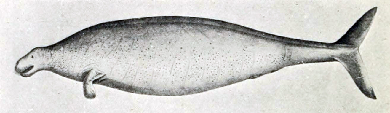
Steller's sea cow (Hydrodamalus gigas).  Drawing by Georg Steller.  Image from Wikimedia.

This week's Challenge was to determine

1.  Are these two animals (the Steller's sea cow and the Steller's jay) named for the same person?  If so, who?  Whatever became of Steller?  

2.  I imagine that these animals were both discovered during an exploratory voyage of some kind.  Can you find out the name and organizer of the voyage that found both the Sea Cow and the jay?   

3.  Can you make a Google Map that shows the voyage of discovery wherein both a sea cow and a blue jay were found?  Ideally, your map would show the path the explorers took and have a couple of markers showing where both the sea cow and jay were discovered (as well as any other discoveries that might be significant).  

1. and 2.  Sea cow AND  jay named for the same person? Found on a voyage?  A:  Yes!  Two quick searches show us that they're both named for Georg Steller.  Wikipedia tells us that he was "Georg Wilhelm Steller (10 March 1709 – 14 November 1746), a German botanist, zoologist, physician and explorer, who worked in Russia and is considered a pioneer of Alaskan natural history."   He gave his name not just to the Steller's sea cow, but also Steller's sea eagle, Steller's jay, Steller's sea lion, and Steller's eider (smallish sea duck that breeds along the Arctic coasts of eastern Siberia and Alaska).  

Steller's eider.  Image from Wikimedia.

Steller's sea eagle.  Image from Wikimedia. 

Steller's sea lion.  Image from Wikimedia.  

Steller traveled to Russia as a physician arriving in November 1734. He met the naturalist Daniel Gottlieb Messerschmidt at the Imperial Academy of Sciences. Two years after Messerschmidt's death, Steller married his widow and learned from his unpublished notes about Vitus Bering’s Second Kamchatka Expedition.  Unfortunately, it had already left Saint Petersburg in February 1733. He volunteered to join the research expeidition and in January 1738 left to catch up with the group's planned exploration of the Kamchatka peninsula. He finally caught up with the main expedition in March 1740. 

Bering summoned Steller to join the voyage to the east in search of America and the strait between the two continents, serving in the role of scientist and physician.  The expedition's two ships became separated, and Bering's ship continued to sail east, expecting to make American landfall soon. Steller, reading sea currents and flotsam and wildlife, insisted they should sail northeast, making landfall in Alaska at Kayak Island in July 1741. Bering wanted to stay only long enough to take on fresh water. Steller argued Captain Bering into giving him more time for land exploration and was granted 10 hours. During this time, as the first non-native to have set foot upon Alaskan soil, Steller became the first European naturalist to describe a number of North American plants and animals, including a jay that became known as Steller's jay.  The first scientific description of the sea otter is contained in the field notes of Steller from 1751.

The sea cow described by (and named for) Steller lasted barely 25 years after it was discovered, a victim of over-hunting by the Russian sailing crews that followed in Bering's wake. In Steller's brief encounter with the bird, he was able to conclude that the jay was a cousin to the American blue jay, a fact which seemed suggested strongly that Alaska was indeed part of North America.


The expedition was a hard one, with many of the crew suffering from scurvy.  Although Steller tried to treat the crew's scurvy with leaves and berries he had gathered, officers declined his proposal. As a results, Steller and his assistant were some of the very few who did not suffer from the ailment. On the return journey, with only 12 members of the crew able to move and the rigging rapidly failing, the expedition was shipwrecked on what later became known as Bering Island. Almost half of the crew had perished from scurvy during the voyage. Steller nursed the survivors, including Bering, but the aging captain couldn't be saved and died from a deficiency of Vitamin C.

On the return trip, Steller came down with an unknown fever, and died in Tyumen, Siberia, trying to get back to St. Petersburg.  

3.  Can you make a map of the expedition?  

By reading this history of Steller and Captain Bering, it gives us an important clue: The name of the expedition.   It's not Steller's expedition--it's Bering's!

So I did a query for: 

     [ map Bering's expedition ] 

and found this lovely map of the entire expedition on the Wikipedia article.  (This is an excerpt of the entire 18th century map which is worth examining.  It is entitled The Russian Discoveries prepared by the London cartographer Thomas Jefferys. This is a reprint published by Robert Sayer in the American Atlas of 1776). 

I ALSO found an already existing map done in Google Maps:  Check out George Stiller's Map of Vitus Bering's Fatal Expedition of 1734.  Many of the icons are clickable and will give you more information about what happened at that spot during the expedition.  

AND Rosemary did this wonderful version of the map that she's given me permission to embed here.   (Be sure to click on the Anchor symbols for nice tidbits about the expedition.)  

I still wanted to find a high resolution map of the expedition, so I did another query:

     [ second kamchatka expedition filetype:kmz OR filetype:kml  ] 

here I'm using the more-or-less official name (in English) for the voyage, and I've added two filetype filters.  A KMZ file or a KML file are files for Google Earth.  I found a couple of them, downloaded them both, and opened them in Google Earth.   (The one I highlight here was created by Tom Kjeldsen in May, 2012.)

As you can see, this map fairly closely follows the The Russian Discoveries map shown above.

You can upload the Russian Discoveries map as a Google Earth overlay, and (within my limits of doing alignment), get something like this:

Or, you could export this to a KML file, and then upload this to your Google Maps:

This isn't a perfect answer to the problem, but there's a lot of good stuff here.  

Search lessons: 

1.  There are maps out there--search first!  

2.  Be sure to remember that Google Earth can import KMZ files and export KML files... which you can then IMPORT into My Maps to create a base layer of placemarks to make the map you really want. 


That's kind of a lot for such a "small" problem, but what a lot of fun!  

Thanks to all of the expert SearchResearchers out there.  (And  a special thanks to Rosemary for sharing her work.)  

Search on! 

Search Challenge (1/28/15): Mapping the discovery of the sea cow and the jay

When I write these Search Challenges....
 I find that they mostly arise from questions that people ask me ("What's that wreck in the water?"), or interesting tidbits that I run across in my non-working life that intrigue me. 

The sadly extinct Steller's sea cow. Image from Wikimedia. 

One such intriguing tidbit I discovered recently is the Steller's sea cow, a large sirenian mammal that's now extinct.  I'd read something about that and wondered if it was somehow connected with the Steller's jay--a common jay in the forests near where I live.   

A non-extinct Steller's Jay.  Photo by Bill Walker. 

Could it be that these two very different animals are both named for the same person?  

Today's Challenge, like all good Challenges, comes in three parts. 

1.  Are these two animals named for the same person?  If so, who?  Whatever became of Steller?  

2.  I imagine that these animals were both discovered during an exploratory voyage of some kind.  Can you find out the name and organizer of the voyage that found both the Sea Cow and the jay?  

3.  Can you make a Google Map that shows the voyage of discovery wherein both a sea cow and a blue jay were found?  Ideally, your map would show the path the explorers took and have a couple of markers showing where both the sea cow and jay were discovered (as well as any other discoveries that might be significant).  

As an example, here's a map showing a portion of the Voyage of the Beagle, Charles Darwin's famous trip around the world that gave him so much data and profoundly influenced his work on evolution.  

From Google Maps Gallery. 

This is a fun challenge full of great surprises.  (Or at least I learned a great deal of fascinating natural and social history in the process.)  It's not difficult, just really, really interesting.  

Search on! 

A quick reflection on the "Where's the lake...?" Challenge

I don't know about you, but in the history of SearchResearch, the "Where's the lake...?" Challenge was probably the toughest Challenge to date.

But it actually wasn't quite what I thought would happen!  I had 3 big surprises in this Challenge.  

1.  SearchResearchers fairly quickly agreed on using Fusion Tables as the main tool for pulling all the data together.  In the discussion group (which was quite active, and very fun to read), the consensus came up fairly quickly. That makes sense, and it's the way I wrote my solution, to follow along in what everyone was doing.    

What I thought was going to happen was that you'd create a mySQL database in the cloud, load up the data, then run your query in that!  

In other words, I tried to write the Challenge so that a "regular" database was needed.  I didn't think that Fusion Tables would be a good solution--but I was wrong.  Obviously, it's quite possible to search a Fusion Table for "All lakes above 8000 feet that have been planted with trout in Northern California."  It was just a matter of applying filters to the data table once it was created by fusing different pieces together. 

I didn't expect that.  But it's a great solution.  Nicely done, team.  


2.  The second thing I didn't expect was that there wouldn't BE ANY lakes that fit all of the criteria.  What do you know?!   (I mean, I knew there were a lot of lakes way high in the California Sierras, and I know that many of them were planted, and when I scanned the list I thought I saw some that I thought fit the bill.  Turns out I misread the dataset when I was creating the problem!) 

As I wrote in the previous blog post, that's part of the reason that you want to use complete data sets (and them put them into Fusion Tables or mySQL so you can query those tools).  This is exactly the kind of thing that search engines are NOT very good at--the very fine grain analysis of data.  A search engine can help you find the data, but then you have to process it a bit yourself, with your own tools.  Metaphorically speaking, the search engine can find you the cow, but you have to make your own sausage.  


3.  I didn't expect all of the back-and-forth steps during my solution.  I realize that my writeup (in three parts) was long and complicated, but I hope you took away one lasting lesson from this:  Even experts have to do a lot of iteration to get the data right.  

In effect, a lot of what I wrote down were all of the "I forgot to include this, let me back up and do it again with this new data" steps.  Normally in classes, the teachers don't show you these steps because they're slightly boring and show what an idiot you are.  (Remember doing proofs in your high school math class?  I realized after a while that nobody really does proofs like that.  Real mathematicians take a lot of forward-and-back steps to figure it out. Everyone goofs.)  

But when I wrote up my solution, I wanted to document all of those intermediate steps as well.  Real data scientists do this all the time, which is why I wanted to write it down, to show you the inner steps that I wish my teachers would have shown me.  

Overall this was a toughie, no doubt about it.  But I hope the search lessons are clear.  If I was to summarize them, I'd say: 

A.  Keep track of your data sources; keep your metadata with the data.  With all of the updates and recasting of the data, it was essential to know where a particular set of data originated.  Keep track of that stuff!  (In FT it's easy--there's a spot for it in the header.  In Spreadsheets, I always add a comment to cell A1 with the metadata.)  

B.  When something takes multiple days to solve, leave yourself a note at the end of the day so you know what you're doing and what's next.  That's why I summarized what the key questions were in each of my posts.  That's basically what I wrote down to keep track of the whole process.  

C.  Check your data.  Check your data.  Check your data.  As you saw, a couple of times I found errors in transcription, or data getting clobbered by accident. (Such as when the lat/longs on Horseshoe Lake were wrong.)  I like to try to view the data in a different way--such as plotting the locations on a map--to see what I can spot.  Spreadsheet computations are often a source of error, so constantly check to make sure that each time you touch the data, you're not accidentally messing it up.  

D.  Keep trying.  This was really a multiple step problem.  Sometimes you just have to stick with it.  

Thanks again to everyone for sticking with the problem.  It was great to see everyone pitching in and contributing.  

Search on! 

Answer: Where's the lake... (Part 3 of 3)

I realize that this is a kind of long process, but stick with me until the end.  It's got a twist ending.  

A quick recap of what we've done over the past couple of days... 

 Post #1 we started to figure out everything that's needed.  Here's what we did:  

1. Find a list of lakes in CA.  Find the USGS GNIS system, and use it to...  

2. Download the GNIS list of lakes, import into a Fusion Table (“Lakes in CA”), convert their LAT, LONG into decimal lat/long. 

3. Find a list of the stocked lakes in CA.  Find the CDFW list. 

4. Download the CDFW list of stocked lakes into a spreadsheet (“Fish planting”) 

5. Merge the “Fishplanting” table with “Lakes in CA” to make “Merge of Lakes…” FT 

6. Check the data.  Create a map of all the Horseshoe Lakes.  Notice that the Horseshoe Lakes are all in the wrong places.  Why?  Make a plan for the next post... 

Post #2 we've got errors--we need to fix them up and find the answer.  

7. Work backwards to discover that the lat/long conversion in step 2 was wrong.  Fix that up and re-merge the tables together. 

8. Map the Horseshoe Lakes again, and check that they’re correct.  (They are now.) 

9. Check ALL of the Horseshoe Lakes in the table and find that the one in Alameda county is missing—why? 

10.  Discover that it’s actually a reservoir, and not in the master list of lakes from GNIS (step 2). 

11.  Go back to GNIS and import a list of all the reservoirs in CA, and re-merge that table into the master list of “CA lakes and reservoirs with extracted lat/longs”  and re-merge everything together. 

12. Now, in the newly re-merged table, notice that all of the Horseshoe Lakes have the same lat/long.  Now what?  Why is this happening?  

13. By looking over the data tables, find that there’s only one Horseshoe Lake that has been planted, the one in Alameda county.  Figure out that the fusing step overwrites ALL of the lakes names “Horseshoe Lake” with the same lat/long value because the lake names are not unique.
 

That gets us up to today’s post.   

Post #3 in which we solve those last problems and find the answer! 

Here's a sketch of what we need to do today.  

Step A. Create the unique IDs by fixing up the table to have a new column of Lake+County name. 

Step B. Re-fuse the tables together to make a new, correct table.

Step C. Filter to see the lakes that have been planted, and in Northern California, AND above 8,000 feet in elevation. 

Step D.  Figure out the surface area of the lakes, and find the lakes that are > 500 acres, above 8,000 feet, AND have been stocked with fish in 2014. 

Step A.  Fix up FT to have Lake+County IDs. 

First, I opened the original spreadsheet for the "Fish Planting" (because you can’t manipulate columns easily in a Fusion Table).  Then, in that spreadsheet I... 

- added a new column (G) called “LakeCounty” which is column C (“Lake name”) concatenated with column B (“County”).   This gives us a new column "LakeCounty" which is unique, and will let us fuse the tables together.  It looks like this: 

Check out the new column on the far right.  That will come in handy in a bit.  

I'll want to fuse this with the fish plantings FT in a minute, but first I need to convert this spreadsheet into a FT first.  Create a NEW FT “Fish Planting Schedule 3” with the newly updated “Fish Planting” spreadsheet.

Now I need to go back to the “CA lakes with extracted lat/longs” spreadsheet  and add a new column (T) that is called “LakeCounty” which is column A (“Lake name”) and concatenate it with column D (“County”).   This will give us a key (that is, the column “LakeCounty”) over which we can fuse our data sets. 

Now, create a new FT from that spreadsheet, and give it the same name “CA lakes with extracted lat/longs”  (There's no confusion here because the first one is a spreadsheet, while this one is a Fusion Table (FT).  

Step B.  Fuse the tables together.  We need to fuse these two FTs -- “Fish planting schedule 3” with the “CA lakes with extracted lat/longs”.  This will give us the planted lakes fused on the key “LakeCounty.” 

The newly merged FTs is “Merge of CA lakes with extracted lat/longs and Fish planting schedule3” 

With me so far?  This table looks like this: 

Note that I've hidden a lot of the extra columns that we don't care about.

NOW we’ve got the Fusion Table we want.  It’s got unique IDs for each lake (“LakeCounty”), along with the correct lat/long, the elevation, and the fish-planting date.  The blank rows on the right (where the yellow marks are) are lakes that were never planted.  Those columns ("Announce Date" etc) all come from the Fish Planting data that was fused with the lakes table.)  

First we look for the lakes/reservoirs in Northern California.  To play it safe, let’s filter on all lakes above latitude 39.0 (that’s roughly the centerline of California).  Click on the Filter button, and let's look at lakes between 39 degrees and 90 degrees of latitude.  (Remember that the correctly extracted latitude is in column LAT1.)  

Then sort by elevation (“Ele(ft)”) and we see this list sorted by elevation.  (Note that I’ve hidden many of the columns that aren’t useful to us now.  Here we see only the relevant columns.) 

Step C.  Filter to see the planted lakes.  And now, in the next-to-last step, we can filter by which lakes have been planted.  Just add a new filter (by clicking on the blue Filter button) and add a filter by FishType = ‘trout’

WHAT?  

There ARE no lakes that have been planted with fish in California that are above 8,000 feet in elevation!

As you can see, there are only 2 planted lakes in northern California, and only 1 of them is even reasonably high (Lake Almanor, at 4505 feet). 

Step D.  Check on the sizes of the lakes.  

Let’s check to see how big these lakes are. 

A quick search for [ Lake Almanor ] tells us that it’s 43.75 sq miles (113.3 km²), or well over 500 acres.  Likewise, a search for [ Baum Lake surface area ] tells us that it’s only 89 acres in size.  It’s nowhere near 500 acres we were looking for.  (And a quick look on the map reveals it’s long and skinny—not a biggish lake at all.) 

So... after all this analysis, we find that Little Rob and Big Jim probably don't actually need the Acetazolamide pills.  (I'm sure you did a search on Acetazolamide and found that it's a commonly used prescription drug for high altitude sickness.)  

But they're clearly headed for the largest, highest lake that's been planted with trout... and that's probably Lake Almanor in Plumas county.  

Map of Northern California showing Lake Almanor between Lassen and Tahoe National Forests

 Search Lessons:  

There are a LOT of lessons here, and I'll discuss some of them in more detail tomorrow.  

But the two biggest lessons are the ones I hope you take away, even if you didn't go through all of the Fusion Table details.  

1.  Sometimes the results aren't quite what you thought.  In this case, because we took the "download all the data and analyze it" approach, we were able to show pretty conclusively that there ARE NO lakes over 8000 feet that are planted with fish.  Just doing a set of queries for this kind of Challenge just doesn't cut it.  This is definitely one of the hardest things to find--a negative result.  But we were able to do it, even if (especially if) the result isn't what you expected. 

2.  Complex search is often a multi-step process.  As you saw, I took a lot of back-and-forth steps along the way, making one table, and then having to go back and modify it to include more information (e.g., adding a unique ID for lake names).  This was a slightly more involved search than usual, but it's not that uncommon a process for sensemaking and data science.  Welcome to data wrangling 101!  

And... to top it all off, while this solution works just fine, it wasn't what I thought you'd do!  (I'm showing you the Fusion Table solution, but there's another way to solve the problem that involves building a database... but we'll tackle that in another month or so.)  

Tomorrow... Reflections on the thought process to solve this Challenge, and my comments on the Discussion group for this problem. 

Searching on! 

Answer: Where's the lake... (part 2 of 3)

Preface:  I know this is kind of a longwinded solution to the problem, but I wrote down all of the steps I took along the way.  "But Dan," I hear you cry, "why not just give us the answer?"  Because I wanted to show all of the steps and mistakes that I made along the way.  This is all to illustrate that sometimes a SearchResearch process takes multiple steps, sometimes going forward, and sometimes backing up to fix errors.  We'll wrap this all up tomorrow with the big conclusion and a set of invaluable search lessons!  

Last week I left off in mid-solution, trying to figure out 4 questions that came up during my research.  Here they are again... 

1.  Why are the lat/longs for the lakes in USGS (FT, Lakes in CA, Fig 12) wrong?  That doesn't make sense--USGS are the people who provided the original data!  

2.  Why are the Horseshoe lakes plotted on the map in Fig 11 all in the wrong place? 

3.  (Important clue) Why is the lat/long of the Horseshoe Lake in Alameda county not the same as any lat/long in the master list?  

4.  (Another important clue) Why do all of the Horseshoe lakes in the Fusion Table of Fig 10 have the same lat/long??  

I'll answer these questions today, and then, once we've got all of our ducks (or fish) in a row, we'll get to the final answer.  

Let's pull up these figures again. Here's figure 12 again.   

Fig 12. List of Lakes in CA in a Fusion Table, filtered by "horse" in the name.

I asked "why are the lat/longs wrong here"?

Here's what I thought was going on.  

I knew that California is mostly at the 37th latitude, and the longitude was mostly around -119 (you can look that up on any map--just drop 37, -119 into a Google Map and you'll end up more-or-less in the middle of California).  

So I wrote a small spreadsheet function to pull off the first 2 digits of the strings in the Latitude column, and the first 3 digits of the Longitude entries, and then use the rest of each string as the decimal part of the lat/long.  (That is, 1190983W would become -119.0983 )

But if you do that, then the coordinates don't actually point to the place they describe!  In other words, the entry for Horse Lake in Sierra county (393912N, 1203930W) would become 39.3912, -120.3930.  If you put that into Google Maps, it's about 59 miles south of the real Horse Lake in Sierra county.  

This puzzled me for a while until I had the bright idea of actually searching for the definition of the lat/long as defined by GNIS.  I did the query: 

     [ GNIS latitude longitude definition ] 

and found the page for "Geonames File Formats."  

I had committed a classic mistake:  I thought I knew what the format was.  And I based my analysis on what I thought.  And I was wrong.  This isn't the format of those numbers at all!

On this page, it says that the lat/long when stored as a "primary latitude" (or longitude) is stored in the DDMMSS format.  (That is, the first two characters are the Degrees, the next two are the Minutes, the last two are the Seconds.)  

I'd assumed they were in decimal lat/long format, not degrees/minutes/seconds format!   

I went back to my spreadsheet and wrote a small converter function to go from degrees/minutes/seconds to decimal.  (It sounds hard, but it's not.  Just extract the minutes, convert to a number and divide by 60.  Same thing for the seconds, but divide by 3600.  Add it all up and you've got your decimal lat/long, suitable for Google Maps. For details, see CA Lakes with extracted lat/longs.  Look at columns K through R.  You can see how I pulled out the middle characters, converted them to numbers, divided by 60 (or 3600) and added them together to give the correct lat/long).  

Now I've got the correct lat/longs.  And when I plot the lakes with the name "Horse" in them, everything looks correct. 

Here's a My Map I made with the lakes that have "horse" in their name.  

So now we've corrected the lat/longs for all the lakes.  And this answers the first two questions: What are the lat/longs "wrong"?  And "Why are the Horseshoe Lakes in Fig 11 in the wrong places?"  

Answer: I messed up the data conversion.  

But now, what's going on in Question 3 (from above)?   (Repeat:  "Why is the lat/long of Horseshoe Lake in Alameda Country not the same as any of the Horseshoe Lakes in the master list?") 

Ah... It's true.  Horseshoe Lake (Alameda) doesn't appear anywhere in the master list of lakes in California.  Why?  

There's a hint in my original question:  "Can you find all of the lakes and reservoirs in California...?"  

A quick search for [ Horseshoe Lake Alameda County ] quickly reveals that it's a reservoir, and the "master list of lakes" doesn't contain all of the reservoirs.  

Okay, so we have to backtrack and find a list of reservoirs and that THOSE into the master list.  

Back to the GNIS system, and this time ask for reservoirs!  

We can get that list of reservoirs, and append it to the bottom of our Lakes in CA spreadsheet and create a new spreadsheet CA lakes and reservoirs with extracted lat/longs.  

There it is--the full list of all Horseshoe Lakes, including Alameda County's reservoir.  

(FWIW, that spreadsheet is 3379 rows long.  A fair number of lakes! But I don't want to think about the number of lakes in Minnesota.)  

And now we're ready to answer the last of our questions for today:  "Why do all of the Horseshoe Lakes in the Fusion Table of Fig 10 have the same lat/long??"  

Fig 10.  Faulty Fusion Table with wrong lat/longs for Horseshoe Lake

As you can see, all of the Horseshoe Lakes are set to 37.57295200, -122.00143000 -- what's up with that?  

What happened is that we fused two tables with non-unique keys.  

That is, we took "Lakes in CA" and fused it with "FishPlantingSchedule2."  

But what happened is that there are (as we see from above) a LOT of lakes named "Horseshoe Lake."  But there's only ONE entry for Horseshoe Lake, and it's the one in Alameda!  

Here, I'm filtering the FishPlantingSchedule2 FT to show me all lakes named "Horseshoe" -- and you can see there's only one, and it's with that lat/long (37.57295200, -122.00143000).  This is kind of whacky.  What's going on? 

Let's step back for a second to see what happened.  

When you fuse two tables together, you're merging them based on a "key" -- in our case, we used the name of the lake as the key.  

Here are the column headings for the "Lakes in CA" FT.  

And here are the column headings for the "FishPlantingSchedule2" FT.  

When you fuse the tables, you have to pick a column to "join."  I chose to fuse (or join) on the "Name" column.  

In essence, the fuse process goes through every row in the "Lakes" table, and looks for a row in the "FishPlanting" table that has a matching name.  

When it does this, it finds all 11 of the "Horseshoe Lake" rows in the "Lakes" table, and joins them with the ONE ROW in the "FishPlanting" table.  In other words, it copies the contents of the "FishPlanting" Horseshoe Lake row into the fused table.  

And it copies the same lat/long into the new table as well.  

Ah ha!  That means that the lat/lon from those columns in the FishPlantingSchedule2 table gets copied into every row of the new fusion table.  

So what we need to do instead is to join on a column that has a unique name for every lake/reservoir.  

See that column labeled "ID" in the Lakes table?  That would be perfect!  That's a unique ID for every feature that GNIS knows about. It would be a perfect column to fuse on because every lake is guaranteed to have a different, unique number. 

Except we don't have the IDs for the lakes mentioned in the Fish Planting table.  Arrgh!  

But don't panic, we can make up our own unique IDs by appending the County name to the name of the lake/reservoir and then join on that unique column.  


BUT.. I'll do that tomorrow.  

Take heart, we're almost done.  

All that's left to do now is: 

1. Create the unique IDs by fixing up the table to have a new column of Lake+County name.  

2. Re-fuse the tables together to make a new, correct table. 

3. Pull the lakes that have been planted, and in Northern California, AND above 8,000 feet in elevation.  

And then we'll tackle the surface area.  (Believe me, after all this, the surface area will be a piece of cake.)  



Hang in there.  Almost to the end!